A long time ago, when applying to one of the unicorns, they gave me a take-home exercise that I remember to this day.
The task was about writing a controller for a remotely-controlled drone, and its controls were accessible over gRPC.
I remember it not just because it was fun, but because I had an eureka moment – in my university, we went through a similar problem, which allowed me to implement the solution right away. That solution was a PID controller.
PID Controllers?
PID Controllers are one of the most widely used control mechanisms in engineering. They adjust a system’s control input to keep a process variable at a desired value while accounting for momentum and avoiding overshoots.
The underlying algorithm is surprisingly simple. The basic idea behind any feedback controller loop is trivial:
- measure the current state
- compare it with the target
- adjust
However, there are various ways for us to utilize that difference between the measured value and the setpoint.
We’ll use a cruise control simulation as our running example, which should make the behavior of each controller variant easy to reason about.
Step 1: Naive Proportional Controller (P)
Let’s say we want to get to and maintain a setpoint of 100 km/h.
double error = setpoint - measured;
The setpoint is our target, measured is where we are right now, and error is the gap between the two.
The most obvious approach is to push hard when we’re far from the target and push gently when we’re close:
record PController(double kp) {

    double compute(double setpoint, double measured) {
        double error = setpoint - measured;
        return kp * error;
    }
}
The controller parameter kp controls how aggressively the controller reacts by making the output proportional to the error. That’s where P comes from.
Let’s see it in action. Simulating those scenarios is actually easier than expected:
- throttle accelerates the car
- drag slows it down (and doesn’t change, at least for now)
Drag’s existence means that the car needs continuous throttle just to maintain speed.
// double TARGET_SPEED = 100.0;
// double DRAG = 0.1;
// double DT = 0.1;
// int STEPS = 1000;

var controller = new PController(1.0);
double speed = 0;

for (int i = 0; i < STEPS; i++) {
    double throttle = controller.compute(TARGET_SPEED, speed);
    speed += (throttle - DRAG * speed) * DT;
    System.out.println(i + ": speed = " + speed);
}
Let’s have a look at the results:
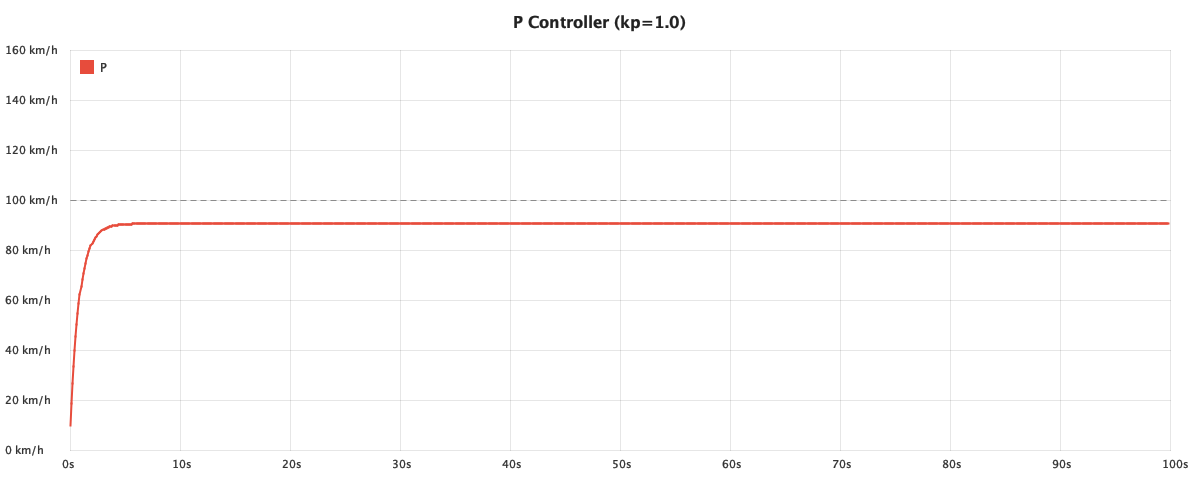
As we get closer to the target speed, the error shrinks, and the throttle decreases, but drag keeps pulling the speed down, and we end up with a phenomenon called steady-state error.
It’s the fundamental limitation of proportional-only control.
We need to address this somehow.
Step 2: Proportional-Derivative Controller (PD)
The problem with the above solution is that it doesn’t acknowledge momentum in any way. It doesn’t care if the error is increasing/decreasing – it sees just the difference.
In order to do something about this, we need to start looking at the error’s rate of change, which means we need to start tracking previous error:
private double previousError;
And then calculate the rate of change (derivative):
double rateOfChange = (error - previousError) / dt;
And incorporate it into the equation:
return kp * error + kd * rateOfChange;
And here’s our new implementation:
class PDController {

    private final double kp;
    private final double kd;

    private double previousError;

    PDController(double kp, double kd) {
        this.kp = kp;
        this.kd = kd;
    }

    double compute(double setpoint, double measured, double dt) {
        double error = setpoint - measured;
        double rateOfChange = (error - previousError) / dt;
        previousError = error;
        return kp * error + kd * rateOfChange;
    }
}
Let’s see it in action:
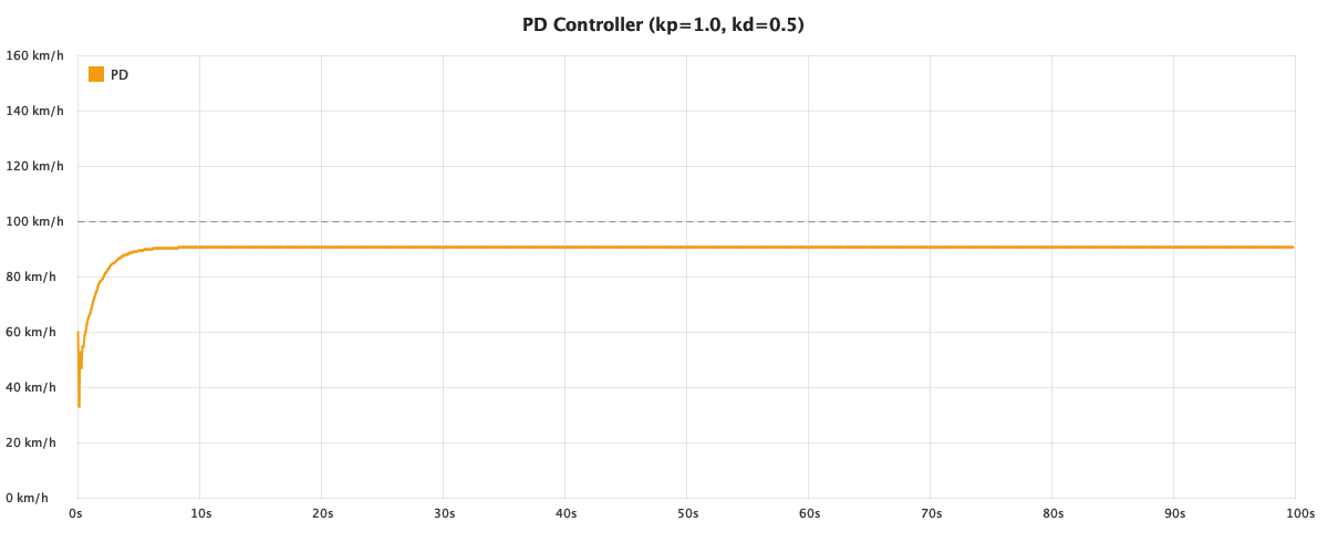
The result is a much smoother response, but it doesn’t help with the core issue much. At the end of the day, the rate of change of a constant error is close to zero, so in the long run, we’re back to the same P-only behavior.
Let’s try something else.
Step 3: Proportional-Integral Controller (PI)
To close that persistent gap, we need something that accumulates error over time.
If you recall calculus, an integral represents the area under a curve. Here, the curve is our error over time, and integral += error * dt is just us summing up tiny rectangles of width dt and height error, so the longer the error persists, the larger the area grows, which results in throttle increase:
class PIController {

    private final double kp;
    private final double ki;

    private double integral;

    PIController(double kp, double ki) {
        this.kp = kp;
        this.ki = ki;
    }

    double compute(double setpoint, double measured, double dt) {
        double error = setpoint - measured;
        integral += error * dt;
        return kp * error + ki * integral;
    }
}
Let’s see it in action: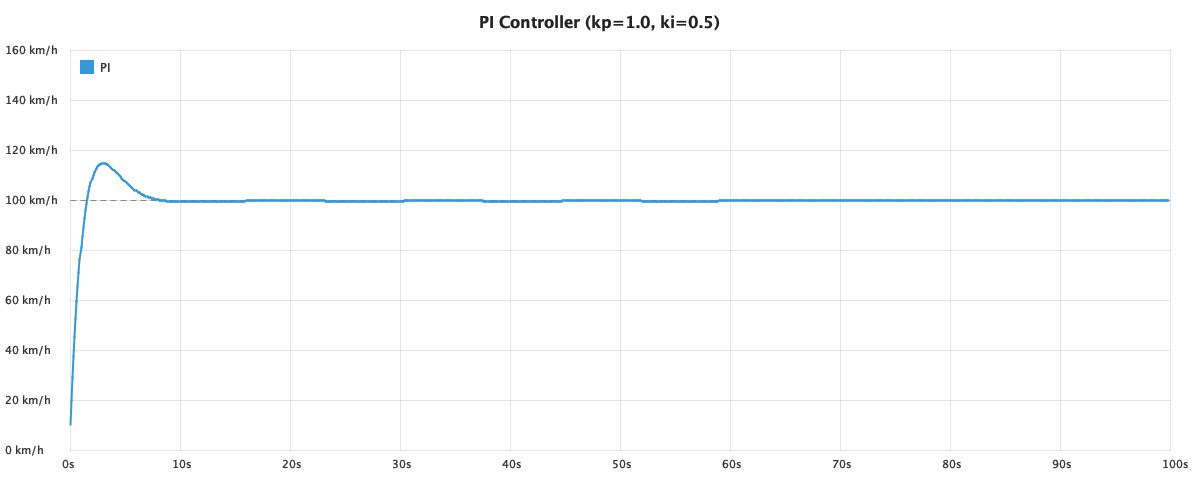
Whoa! This actually works! Our car actually reaches 100km/h! Our integral makes sure that as long as there’s error, throttle adjusts, so the controller never settles below/above the target.
However, if you look closely, you can see that it oscillates a bit.
This is already pretty good for many real-world systems where overshoot isn’t a problem.
However, there’s one more thing we need to address. Our PI controller has no output limits so let’s add output clamping:
return Math.clamp(output, outputMin, outputMax);
And let’s see what happens.
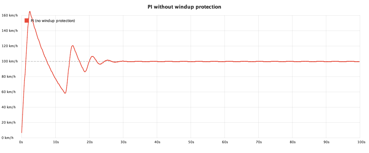
Whoa! that’s actually much worse! That massive overshoot and oscillation is caused by a phenomenon called integral windup.
During startup, the car is at 0 km/h and the target is 100 km/h. The error is large, and the integral term keeps accumulating it every time step so it just piles up silently.
When the car reaches 100 km/h, the integral has grown huge. Even though the error is now zero, the accumulated integral causes massive overshoot. The controller then has to offload (or rather unwind) all that accumulated integral.
The fix is straightforward: when the output hits the min/max limits, we undo the last integral accumulation:
if (output > outputMax) {
    accumulatedError -= error * dt;
    return outputMax;
}
if (output < outputMin) {
    accumulatedError -= error * dt;
    return outputMin;
}
This way, the integral only accumulates when the controller’s output is actually being used.
The difference is drastic:
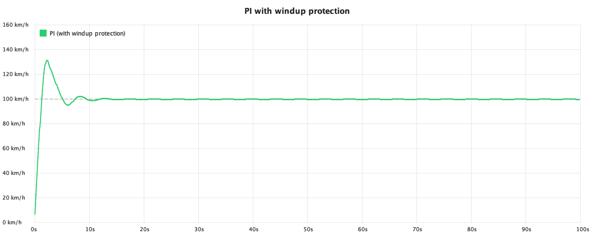

But our controller still oscillates more than it should. Let’s bring back the derivative term.
Step 4: Full PID Controller
In order to end up with the ultimate solution, we need to combine all three approaches into a single controller that eliminates steady-state error and dampens overshoot.
We already know about windup protection, so let’s bake it in from the start:
class PIDController {

    private final double kp;
    private final double ki;
    private final double kd;
    private final double outputMin;
    private final double outputMax;

    private double accumulatedError;
    private double previousError;

    PIDController(double kp, double ki, double kd, double outputMin, double outputMax) {
        this.kp = kp;
        this.ki = ki;
        this.kd = kd;
        this.outputMin = outputMin;
        this.outputMax = outputMax;
    }

    double compute(double setpoint, double measured, double dt) {
        double error = setpoint - measured;

        accumulatedError += error * dt;
        double changeRate = (error - previousError) / dt;
        previousError = error;

        double output = kp * error + ki * accumulatedError + kd * changeRate;

        if (output > outputMax) {
            accumulatedError -= error * dt;
            return outputMax;
        }
        if (output < outputMin) {
            accumulatedError -= error * dt;
            return outputMin;
        }
        return output;
    }
}
Each term handles a different aspect of the control problem now, but the final result doesn’t seem significantly better than the previous result:

Tuning
The implementation of PID is easy, but it’s the tuning that’s hard. The right values depend entirely on the system being controlled, and the trade-offs between responsiveness, overshoot, and stability.
Let’s see what a difference tuning makes for our cruise control. Here are four parameter sets, all using the same PID controller:
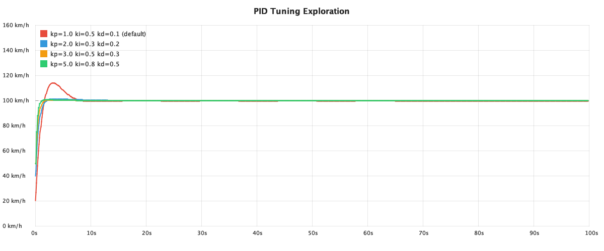
So how did I do it? Well, good old trial and error. While this might sound disappointing, quite often it’s the most pragmatic choice in real life systems. However, for formal approaches, look into the Ziegler-Nichols method or Cohen-Coon tuning.
Here are a few tips to make your trial and error easier:
- p controls how aggressively system responds, but if you increase it too much, you’ll get oscillations
- i removes steady-state offset, but too much of it makes the system sluggish
- d smoothes the response, but can amplify noise
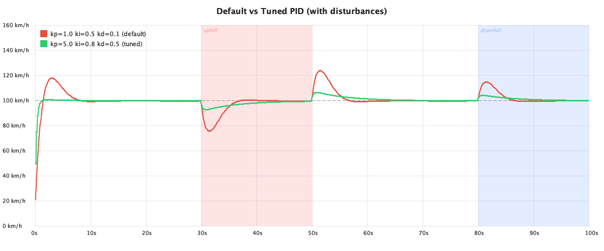
As a bonus, here’s our tuned controller running though disturbances:
Source Code
As always, the source code is available on GitHub.